Firmware/Linear Acceleration

WIP: This is a Work In Progress

Physics of Motion

Velocity

<math>V=dx/dt</math>

A change in position is motion. The speed of that change is velocity. Velocity is the first derivative of position with respect to time. That's why velocity is measured as distance/time.

Acceleration

<math>A=dv/dt</math>

A change in velocity is acceleration. Acceleration is the first derivative of velocity with respect to time. That's why acceleration is measured as <math>distance/time^2</math>.

Jerk

<math>J=da/dt</math>

A change in acceleration is called "jerk". Jerk is the first derivative of acceleration, the 2nd derivative of velocity, and the third derivative of position. Jerk is measured as <math>distance/time^3</math>.

Note: this is not the "jerk" value commonly used to smooth out movements on some firmware in the community.

Extruder pressure management

(FIXME: say a few words about how to control the extruder stepper while the other axes are accelerating. Perhaps a summary of "yet another firmware - pressure management / acceleration" and other emails in that thread.)

Trajectory Planning

Trajectory planning is the process of determining how to move the axes to achieve a desired motion or displacement. Higher speeds are possible on stepper motors only through acceleration. The math required to determine stepper times to effect an accelerated motion involves calculus. Some of this calculus is not algebraically solvable.

Constant Acceleration

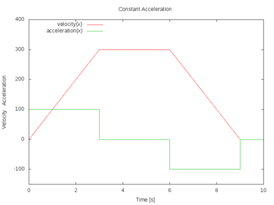
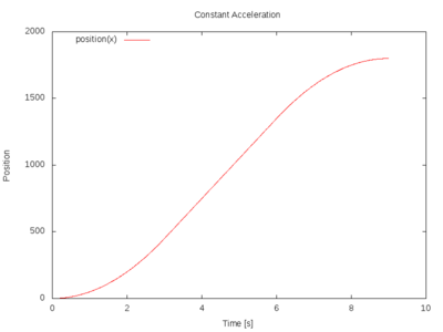
To move the print head correctly, we need to convert acceleration into velocity and velocity into position. Most firmware uses Constant Acceleration. It is mostly good enough and the math used to turn acceleration and time into step timing estimates is simpler than that for variable acceleration planning. The constant acceleration results in a strictly linear velocity profile during the entire acceleration/deceleration phases. This allows much of the math required for the acceleration to be performed in advance of beginning the move.

Linear Acceleration

Velocity planning using linear acceleration requires slightly more complicated math to calculate the stepper timings. It is difficult or impossible to do the required math in real-time on most microcontrollers. There are methods to estimate the correct values, but the precise answer can be attained only analytically (trial and error). There are small errors which accumulate over time when estimations are used, but these can be corrected by determining the error during the movement and compensating for it. More interestingly we can ignore the slight errors in precise step-time and simply ensure that we continue to hit each desired step-time within an acceptably small window.

Curved Acceleration

The velocity path can be calculated on the fly as the piece-wise integration of some linear acceleration value, or it can be a pre-calculated linear velocity ramp, the integral of some constant acceleration value. Often a linear approximation to some complex curve is good enough for our needs.

I am hoping to use it to approximate the velocity curve discussed in this paper (PDF) on exponential velocity planning. The main goal of this complex exponential acceleration planning is to produce smooth, continuous movements free of sudden acceleration changes (jerk). But there are some other interesting ideas to come out of this paper, too.

Infinite jerk

The problem with constant acceleration is infinite jerk. When you go from zero acceleration to max acceleration in zero time, you experience infinite jerk. It's not really infinite, because real physics gets in the way. But the software tries to impart infinite jerk, and the hardware does its best to comply.

Any time the acceleration curve is discontinuous (broken), there is an instantaneous (theoretically infinite) jerk imparted on the machine. This causes stress on the machine parts and over time can damage or wear out the hardware prematurely.

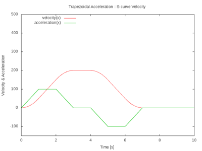
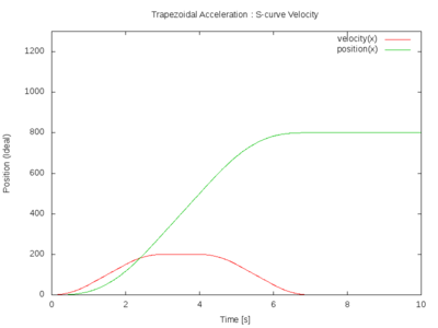
One way to solve this is to use a trapezoidal acceleration profile. In this profile acceleration is a continuous function, but its slope, aka "Jerk", is not. But Jerk is then constant, at least, and not infinite. The resulting velocity profile is smoothed out, and our position plan is even smoother.

<image of constant Jerk, trapezoidal acceleration, smooth velocity>

Algorithms

Stepper motor approximation

<Discussion of the Austin paper>

Manual integration

Here I plan to present a method to achieve linear acceleration through iterative real-time integration of the velocity curve. What we want to do is to calculate the precise time of the next step of the stepper motor. We cannot calculate this value exactly in real-time, but we can estimate it, and we can measure when the real moment has passed. If we do this frequently enough then the window within which we will actually step will be acceptably small that the physics of the motor itself will hide our mistakes; inductance and microstepping are quite forgiving.

<image showing estimated step time, true "ideal" step time, and measured error>

By estimating the next step time in advance, we get a measure of how much slack time is available to perform other tasks (processing g-code, reading thermistors, etc.). As the moment nears when a step needs to occur, we can look to see how much movement should have occurred so far. If it is enough to warrant a step, we can step. If it does not yet add up to a whole step, we can delay a little more and check back later. In fact, if we are really clever, we can determine how _much_ later we should check back, thus refining our estimate. Doing this sort of estimate refinement well can reduce the number of re-estimations we need to do.

<image showing estimated step time, estimated refinements, ideal step times, and real step times; also show piece-wise "area under the curve" measurement of each step>

In effect we perform the analytical calculus needed to determine how movement _should have_ occurred. If we do this often enough (Teacup Firmware uses a 2ms "background" timer for such tasks) we can adjust our velocity in near-real time to match a planned velocity path.

<image of constant acceleration and resulting velocity curve>

Exponential velocity planning

A paper presented in the IEEE in 2013[1] proposed an exponential velocity planning method. Read the paper for all the details. In a nutshell it suggests that a function can be chosen whose first, second, and third derivatives are all continuous curves. Using this function to plan movements therefore leads to smooth acceleration and jerk profiles as well. Detailed analysis of these functions was done and simplified methods to normalize the curve to fit various velocity, acceleration and jerk limits were discovered. Most of the complex math can be solved in advance so the method can be implemented in real time.

Displacement time

A novel idea I learned from this paper involved their treatment of displacement time, Td. Td is the amount of time required to make a move. It's quite simple, really. But the authors of this paper discovered some interesting ways to play with this notion. Here's a simplified description:

Td is the amount of time required to make a move at some velocity, Vmax. The fastest movement minimizes Td by completing the entire move at Vmax. That is, Td = dx / Vmax

We can't really do that because we have to deal with acceleration and momentum and the real world. But let's use this minimum Td as as a lower bound of our movement time.

• Vmax: movement velocity, expressed as distance/time.
• dx: Distance to move
• Td = dx / Vmax = distance / (distance / time) = time

As an example, if we wish to move 40mm and our velocity Vmax is 120mm/sec, then our ideal travel time (displacement time) is given as:

 Td = 40mm / (120mm / sec) = (40 / 120) sec = 1/3 sec

This is all very basic. But what happens when we add in acceleration? Things get so complicated. There is often much math involved. You will find mechatronics papers discussing the 7 movement phases of an accelerated motion, and the 21 equations that must be solved to determine the movement in each phase. Whole books are written on this.

But what I learned from this paper is that it is much simpler than this if we rely on symmetrical acceleration and deceleration, which we do. Here's the interesting part.

<image> This a graph of the "ideal" motion where all travel occurs at Vmax. It's a rectangle. Rectangles are easy, right? Side * side = area. Area in this case is 40mm^2. The "y" side is 120mm/sec. So how big is the "x" side (time)? 40mm / 120mm/sec = 1/3 sec, or 0.3333 seconds.

<image> What happens when we introduce acceleration? In the simple case of constant acceleration, we have a trapezoidal velocity. That means our velocity curve forms a triangle for the acceleration at the start of the move and another triangle for our deceleration at the end of our movement. In the middle we managed to reach Vmax for some period of time. That's called the cruising period, or Tc. Note that it's important to be able to calculate Tc in advance so we know when to begin our deceleration. If we begin decelerating too soon, we will not complete our move. If we begin too late, we will not be able to stop our move at the desired position. We must begin decelerating at _exactly_ the right moment.

<image trapezoidal velocity with shaded areas for Ts, Tc and Ts> Since we didn't get to go top speed the whole time, our motion time is longer than 1/3 of a second. How long it is depends on how steep our velocity is (acceleration). But notice that the area under the curve is the same. The area under the curve is our position change, our dx.

Consider three areas of our curve. Ts = startup time when we were accelerating Tc = cruise time during which we travel at Vmax Te = end time when we have completed our travel

What about the deceleration time? It turns out that because our deceleration and acceleration profiles are symmetrical that it is simple to calculate when to begin decelerating. It is Te - Ts.

How do we calculate Te? Te = Td + Ts.

So Td is actually our deceleration start time.

  Te = Td + Ts
  Te - Ts = (Td + Ts) - Ts 
  Te - Ts = Td

This works because our triangles are identical; the area of a triangle is 1/2 height * base. So, two triangles add up to our ideal travel time graph again.

We can make this relationship work for more complicated profiles which do not use triangles. The paper glosses over that a bit, but it makes use of it. Look there if you want to understand it from the primary source. But the basic idea is so simple. We create our deceleration profile as the inverse of our acceleration profile, no matter what they look like. To make this inverse, we simply subtract our acceleration profile from Vmax when we want to begin decelerating. Where do we want to begin decelerating? At Td = Te - Ts. And Td = dx / Vmax.

<image of complex velocity profile accelerating and decelerating>

Linear approximation

Discussion of linear approximation methods to map velocity or acceleration profiles.

Movement joining

Consider two sequential movements, the first from A to B, and the second from B to C.

A -> B -> C

To perform an accelerated movement accurately from point A to point B in a straight line on multiple axes requires a careful coordination of each axis relative to all the others. This coordination must be done while also respecting the mechanical limits of each axis (e.g. maximum acceleration, velocity and jerk). An accelerated movement which arrives exactly at point B and then continues on to point C without stopping will experience severe Jerk if the <math>\angle ABC</math> is not at or very close to zero. This is because the velocity for such a movement will necessarily change instantaneously at B in order to keep moving on to C at a different angle. An instantaneous change in velocity requires an infinite (impossible) acceleration and so is not practical.

<math>da = dv/dt, dt=0</math>

A change in velocity requires a change in acceleration relative to the time involved. If the change in velocity, dv, is large and the time allowed for the change to occur is small, the change in acceleration, da, becomes even larger. If the time allowed for the transition is zero, the change in acceleration becomes infinite.

There are many ways to join movements. Here are just a few.

Do not accelerate

There must be some non-zero velocity we can achieve "instantly" from a velocity of zero. If there were not, we would not be able to move at all. On stepper motors with small masses like on a RepRap, this velocity is not as small as it might seem. This is our primary velocity which is the result of our fastest possible, reliable, first step of the stepper motor. Call this V-prime (V').

If we never move our axes faster than 1/2 V', then no acceleration is required. It becomes trivial to change speeds at B because every step could be our last step and the mechanics would be ok. We would reliably stop at that point. We can therefore continue from that point at any speed less than 1/2 V' safely. The change in velocity at B will always be less than V', no matter what the new velocity is.

 <math>dv_B < V'</math>

Why 1/2? Why can't you move at V'?

The answer is that if the sign of the velocity from A->B, <math>V_{AB}</math>, is different (opposite) of the sign from B->C, <math>V_{BC}</math>, then you may have dv which is equal to the sum of those two speeds. <math> dv = | V_{AB} - V_{BC} | < 2 * V'</math>

There are ways to deal with this, but they are not interesting here and become more like acceleration anyway.

But V' is interesting. Remember it for later.

Come to a full stop between each move

The simplest way to join two accelerated movements is not to join them. Begin each movement from a full stop at velocity zero, accelerate to speed, and then decelerate to a full stop at velocity zero again. This is the cleanest way to move accurately from point to point, but it is slow and it does impose a lot of Jerk on the mechanics -- even if kept to the acceptable maximum -- since every single movement involves a full start from zero and full stop to zero.

Advantages: Simple and accurate

Disadvantages: Slow and jerky

Minimize or ignore the problem

Find dv, the velocity difference between the two moves.

<math>dv = | V_{AB} - V_{BC} |</math>

If dv < V', you may safely join the moves.

If dv > V', then you must decelerate one or both velocities until dv <= V'.

This method should be accurate if V' is chosen carefully. I think this is what some firmware calls "Jerk", but it is really a velocity value. It is only considered as a velocity delta, so it can be considered an acceleration value. But the time involved, dt, is usually considered to be constant, so the value devolves to velocity again. What should be limited here is the Jerk (the real one), but that is too complicated to calculate in real-time. Also, so long as the speeds are low, dt is nearly constant anyway and it is safe to ignore it. However, the V' which is safe at slow speeds is not safe at high speeds. So either V' has to be chosen conservatively to cover the high speed moves, or else the maximum safe Jerk (da/dt) is likely to be exceeded, resulting in movement errors, aka lost steps, overshoot or position error.

Advantages: Accurate; Safe and simple if V' is chosen carefully.

Disadvantages: More accurate at some speeds than at others; Difficult to tune properly.

Trade accuracy for speed

Suppose you could get very close to point B without actually touching it. How accurate do you need to be, really? If you can accept a certain amount of error in your high-speed moves, you can trade accuracy for speed.

<image Actual positions; error positions; relative velocity>

It is certainly possible to keep a high speed while passing by point B if you allow your hardware to miss point B entirely. There are many methods to calculate this sort of path, and there is no complete list of all of them. But following are some examples.

Trapezoidal velocity joining

Like EMC2 See http://wiki.linuxcnc.org/cgi-bin/wiki.pl?Trapezoidal_Velocity_Profile_Trajectory_Planner

Acceleration / Deceleration merging

Like exponential paper describes.